Hyperfunction
00.26
Formulation
A hyperfunction on the real line can be conceived of as the 'difference' between one holomorphic function on the upper half-plane and another on the lower half-plane. That is, a hyperfunction is specified by a pair (f, g), where f is a holomorphic function on the upper half-plane and g is a holomorphic function on the lower half-plane.
Informally, the hyperfunction is what the difference f − g would be at the real line itself. This difference is not affected by adding the same holomorphic function to both f and g, so if h is a holomorphic function on the whole complex plane, the hyperfunctions (f, g) and (f + h, g + h) are defined to be equivalent.
Definition in one dimension
The motivation can be concretely implemented using ideas from sheaf cohomology. Let  be the sheaf of holomorphic functions on C. Define the hyperfunctions on the real line by
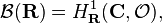
the first local cohomology group.
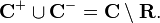
Concretely, let C+ and C− be the upper half-plane and lower half-plane respectively. Then
so
![H^1_{\mathbf{R}}(\mathbf{C}, \mathcal{O}) = \left [ H^0(\mathbf{C}^+, \mathcal{O}) \oplus H^0(\mathbf{C}^-, \mathcal{O}) \right ] /H^0(\mathbf{C}, \mathcal{O}).](http://upload.wikimedia.org/math/b/7/1/b719e91dae08dba88413cd02e9c88145.png)
Since the zeroth cohomology group of any sheaf is simply the global sections of that sheaf, we see that a hyperfunction is a pair of holomorphic functions one each on the upper and lower complex halfplane modulo entire holomorphic functions.
Examples
- If f is any holomorphic function on the whole complex plane, then the restriction of f to the real axis is a hyperfunction, represented by either (f, 0) or (0, −f).
- The Dirac delta "function" is represented by
 . This is really a restatement of Cauchy's integral formula.
- If g is a continuous function (or more generally a distribution) on the real line with support contained in a bounded interval I, then g corresponds to the hyperfunction (f, −f), where f is a holomorphic function on the complement of I defined by
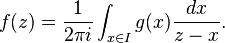
- This function f jumps in value by g(x) when crossing the real axis at the point x. The formula for f follows from the previous example by writing g as the convolution of itself with the Dirac delta function.
- If f is any function that is holomorphic everywhere except for an essential singularity at 0 (for example, e1/z), then (f, −f) is a hyperfunction with support 0 that is not a distribution. If f has a pole of finite order at 0 then (f, −f) is a distribution, so when f has an essential singularity then (f,−f) looks like a "distribution of infinite order" at 0. (Note that distributions always have finite order at any point.)
Posting Komentar